The performance of new sensors and system configurations opens an extended new field of applications. Now also small-scale mass variations in the Earth system might be observed. In this project we study how big mass variations of different origin (e.g. atmosphere, non-tidal and hydrology) are and how much they affect the various gravity field quantities observed by new sensors.
In order to separate different signals, we are using the approach from Farrell (1972) to calculate changes in gravity from modeled mass variations. These models have high spatial and temporal resolution. For example, the input for non-tidal ocean loading is the coastDat2 data created by the Helmholtz-Zentrum Geesthacht. It covers the North Sea, Baltic Sea and the northern Atlantic. Figure 01 shows water height variations during the 2008 storm ‘Emma’. Due to this storm, gravity in Hannover was changed by 14 nm/s2.
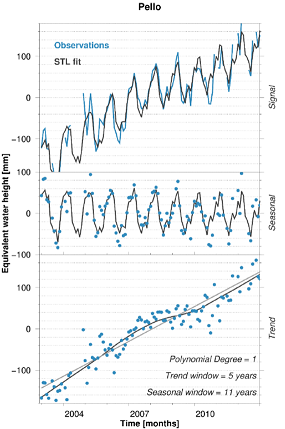
In Fennoscandia much of the time-variable gravity signal is dominated by hydrology (seasonal signal) and post-glacial rebound (PGR) (trend signal). In order to separate these two distinct signal types, seasonal and trend adjustment using locally weighted regression (STL) is used. It is a non-parametric method that applies two different moving windows, one for the seasonal signal and the other for the trend, to estimate the two signals without the signals leaking into each other. This method handles non-stationary signals and captures changes in trend and seasonal behavior.
The project also addresses the problem of de-aliasing of satellite gravity data, i.e. the reduction of high-frequency mass variations during data processing. In order to get a first-hand feeling of aliasing problems and de-aliasing strategies, we are studying ocean-tide aliasing. We use noise-free simulated data, where only the static gravity field and ocean-tide models are used. This is done to quantify the upper bound of the ocean-tide aliasing error.


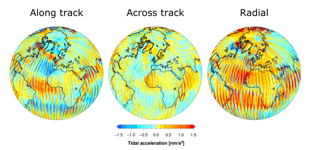
Figure 03: Depiction of residual ocean-tide accelerations in the local instantaneous relative reference frame due to 18 major tidal constituents. It clearly demonstrates the observation geometry of GRACE. The along track and radial components have more signal than the across track component of the differential acceleration vector.
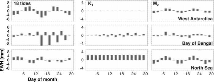
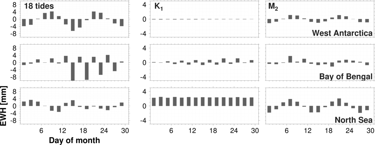
One of the promising strategies for reducing the aliasing errors is the Wiese approach. In general, only monthly estimates of the time-variable gravity field are computed, but in the Wiese approach, low-degree (long wavelength) sub-monthly (usually daily or two-day) solutions are co-parameterized. Since ocean-tides have higher frequencies (diurnal and semi-diurnal) than the sub-monthly solutions, Wiese approach does not mitigate ocean-tides. However, it allows for retrieving the long wavelength ocean-tide aliasing signal as shown in figure 04.


Figure 04: Time-series of the ocean-tide aliasing obtained by parameterizing a 2-day 10-degree solution in the Wiese approach. We can clearly see aliasing periods of the M2 (13 days) tide and it dominates the ocean-tide aliasing signal. Since the K1 tide aliases into a 7.5 year period, we do not see much change in the time-series.
Principal Investigator
Schneiderberg 50
30167 Hannover


